How Roblox Reduces Spark Join Query Costs With Machine Learning Optimized Bloom Filters

Abstract

Every day on Roblox, 70 million users engage with millions of experiences, totaling 16 billion hours quarterly. This interaction generates a petabyte-scale data lake, which is enriched for analytics and machine learning (ML) purposes. It’s resource-intensive to join fact and dimension tables in our data lake, so to optimize this and reduce data shuffling, we embraced Learned Bloom Filters [1]—smart data structures using ML. By predicting presence, these filters considerably trim join data, enhancing efficiency and reducing costs. Along the way, we also improved our model architectures and demonstrated the substantial benefits they offer for reducing memory and CPU hours for processing, as well as increasing operational stability.

Introduction

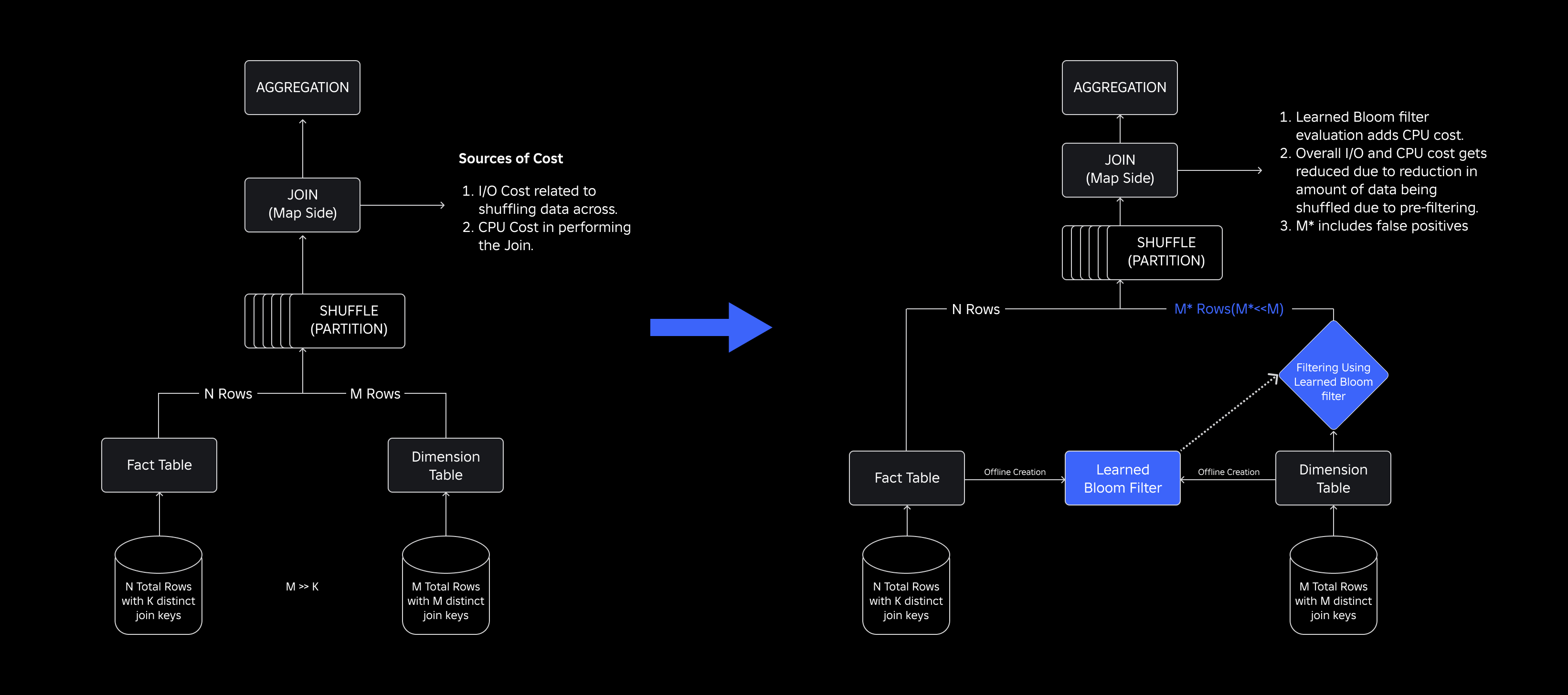
In our data lake, fact tables and data cubes are temporally partitioned for efficient access, while dimension tables lack such partitions, and joining them with fact tables during updates is resource-intensive. The key space of the join is driven by the temporal partition of the fact table being joined. The dimension entities present in that temporal partition are a small subset of those  present in the entire dimension dataset. As a result, the majority of the shuffled dimension data in these joins is eventually discarded. To optimize this process and reduce unnecessary shuffling, we considered using Bloom Filters on distinct join keys but faced filter size and memory footprint issues.

To address them, we explored Learned Bloom Filters, an ML-based solution that reduces Bloom Filter size while maintaining low false positive rates. This innovation enhances the efficiency of join operations by reducing computational costs and improving system stability. The following schematic illustrates the conventional and optimized join processes in our distributed computing environment.

Enhancing Join Efficiency with Learned Bloom Filters

To optimize the join between fact and dimension tables, we adopted the Learned Bloom Filter implementation. We constructed an index from the keys present in the fact table and subsequently deployed the index to pre-filter dimension data before the join operation. 

Evolution from Traditional Bloom Filters to Learned Bloom Filters

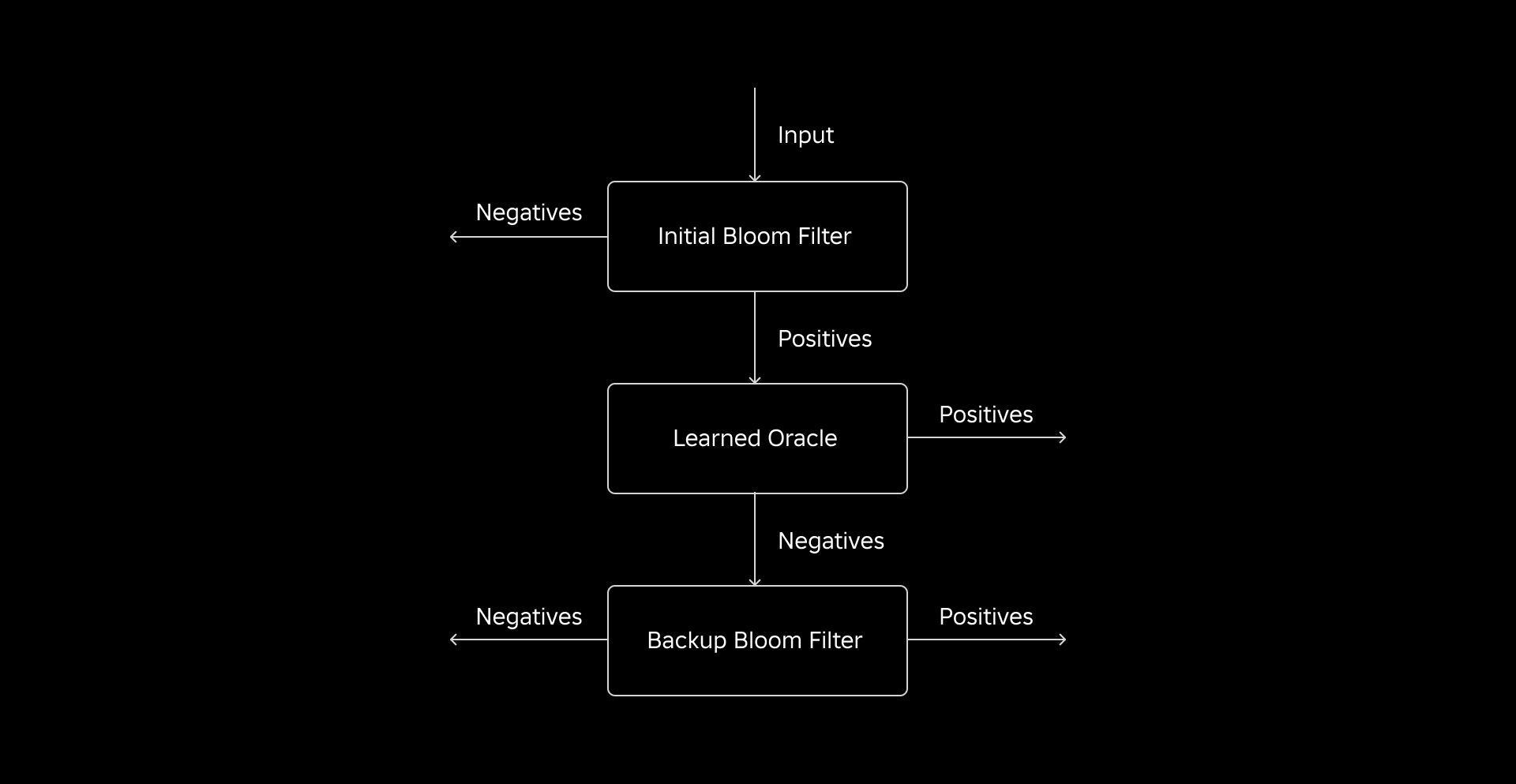
While a traditional Bloom Filter is efficient, it adds 15-25% of additional memory per worker node needing to load it to hit our desired false positive rate. But by harnessing Learned Bloom Filters, we achieved a considerably reduced index size while maintaining the same false positive rate. This is because of the transformation of the Bloom Filter into a binary classification problem. Positive labels indicate the presence of values in the index, while negative labels mean they’re absent.

The introduction of an ML model facilitates the initial check for values, followed by a backup Bloom Filter for eliminating false negatives. The reduced size stems from the model’s compressed representation and reduced number of keys required by the backup Bloom Filter. This distinguishes it from the conventional Bloom Filter approach. 

As part of this work, we established two metrics for evaluating our Learned Bloom Filter approach: the index’s final serialized object size and CPU consumption during the execution of join queries. 

Navigating Implementation Challenges

Our initial challenge was addressing a highly biased training dataset with few dimension table keys in the fact table. In doing so, we observed an overlap of approximately one-in-three keys between the tables. To tackle this, we leveraged the Sandwich Learned Bloom Filter approach [2]. This integrates an initial traditional Bloom Filter to rebalance the dataset distribution by removing the majority of keys that were missing from the fact table, effectively eliminating negative samples from the dataset. Subsequently, only the keys included in the initial Bloom Filter, along with the false positives, were forwarded to the ML model, often referred to as the “learned oracle.” This approach resulted in a well-balanced training dataset for the learned oracle, overcoming the bias issue effectively.

The second challenge centered on model architecture and training features. Unlike the classic problem of phishing URLs [1], our join keys (which in most cases are unique identifiers for users/experiences) weren’t inherently informative. This led us to explore dimension attributes as potential model features that can help predict if a dimension entity is present in the fact table. For example, imagine a fact table that contains user session information for experiences in a particular language. The geographic location or the language preference attribute of the user dimension would be good indicators of whether an individual user is present in the fact table or not.

The third challenge—inference latency—required models that both minimized false negatives and provided rapid responses. A gradient-boosted tree model was the optimal choice for these key metrics, and we pruned its feature set to balance precision and speed.

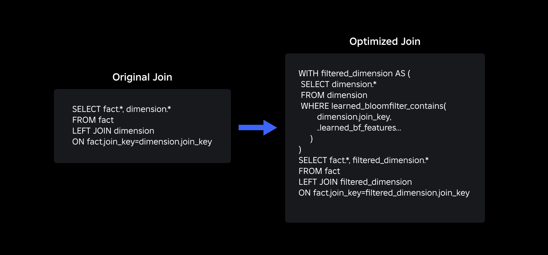
Our updated join query using learned Bloom Filters is as shown below:

Results

Here are the results of our experiments with Learned Bloom filters in our data lake. We integrated them into five production workloads, each of which possessed different data characteristics. The most computationally expensive part of these workloads is the join between a fact table and a dimension table. The key space of the fact tables is approximately 30% of the dimension table. To begin with, we discuss how the Learned Bloom Filter outperformed traditional Bloom Filters in terms of final serialized object size. Next, we show performance improvements that we observed by integrating Learned Bloom Filters into our workload processing pipelines.

Learned Bloom Filter Size Comparison

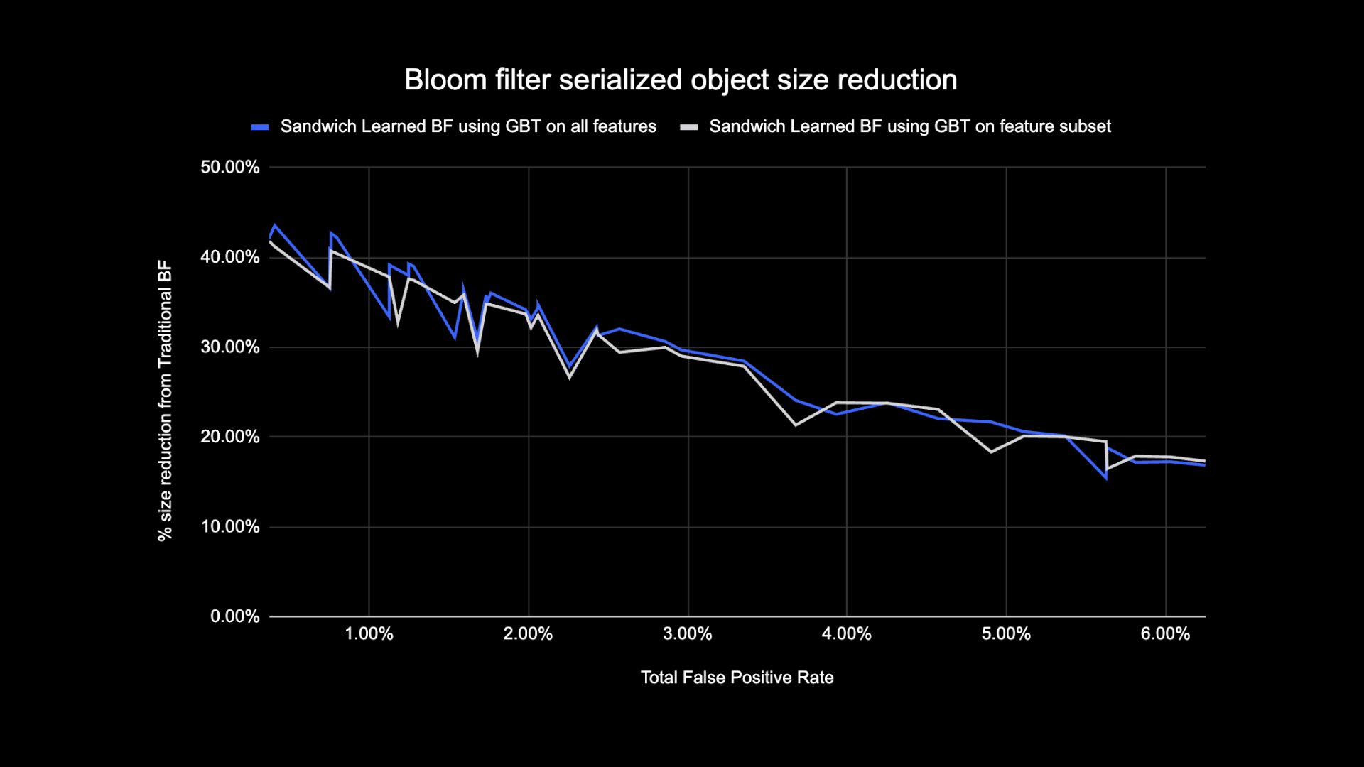
As shown below, when looking at a given false positive rate, the two variants of the learned Bloom Filter improve total object size by between 17-42% when compared to traditional Bloom Filters.

In addition, by using a smaller subset of features in our gradient boosted tree based model, we lost only a small percentage of optimization while making inference faster.

Learned Bloom Filter Usage Results 

In this section, we compare the performance of Bloom Filter-based joins to that of regular joins across several metrics. 

The table below compares the performance of workloads with and without the use of Learned Bloom Filters. A Learned Bloom Filter with 1% total false positive probability demonstrates the comparison below while maintaining the same cluster configuration for both join types. 

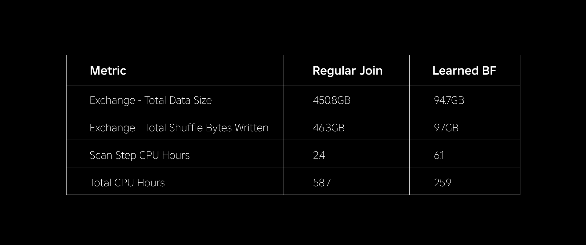
First, we found that Bloom Filter implementation outperformed the regular join by as much as 60% in CPU hours. We saw an increase in CPU usage of the scan step for the Learned Bloom Filter approach due to the additional compute spent in evaluating the Bloom Filter. However, the prefiltering done in this step reduced the size of data being shuffled, which helped reduce the CPU used by the downstream steps, thus reducing the total CPU hours.

Second, Learned Bloom Filters have about 80% less total data size and about 80% less total shuffle bytes written than a regular join. This leads to more stable join performance as discussed below. 

We also saw reduced resource usage in our other production workloads under experimentation. Over a period of two weeks across all five workloads, the Learned Bloom Filter approach generated an average daily cost savings of 25%, which also accounts for model training and index creation.

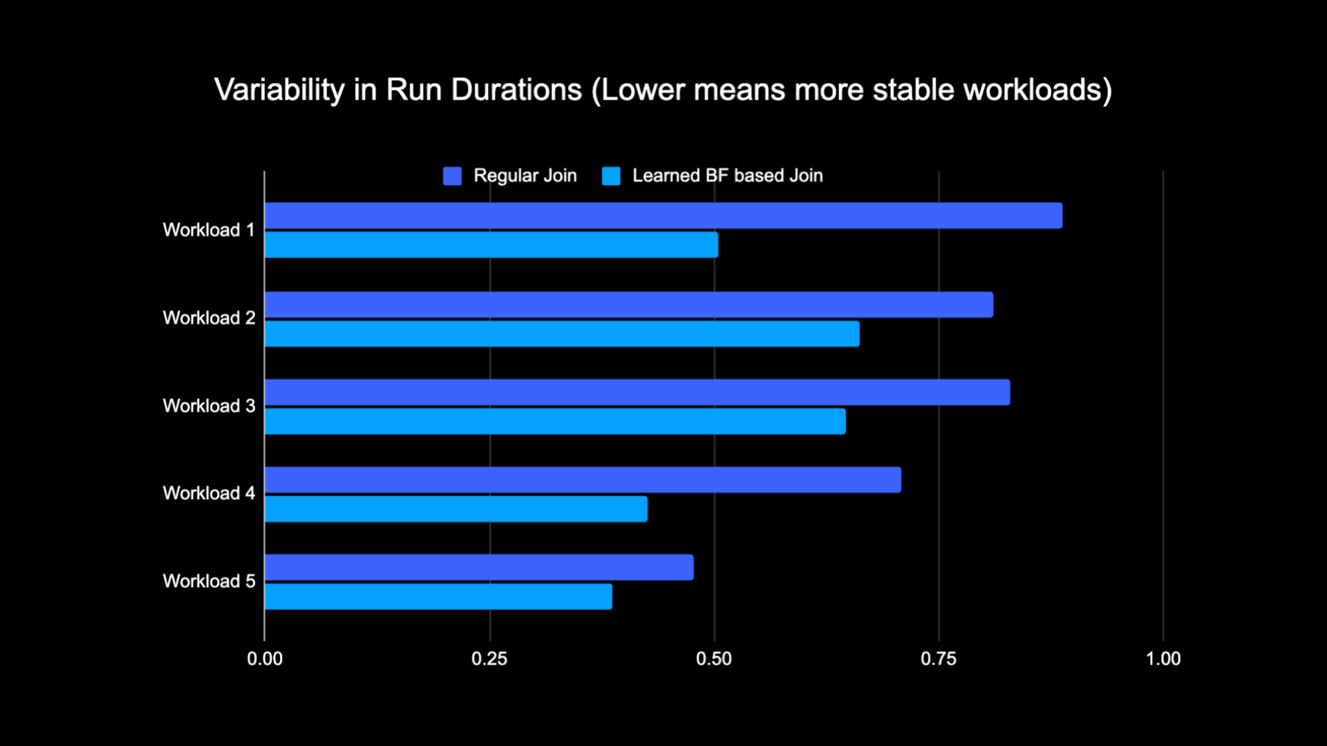
Due to the reduced amount of data shuffled while performing the join, we were able to significantly reduce the operational costs of our analytics pipeline while also making it more stable.The following chart shows variability (using a coefficient of variation) in run durations (wall clock time) for a regular join workload and a Learned Bloom Filter based workload over a two-week period for the five workloads we experimented with. The runs using Learned Bloom Filters were more stable—more consistent in duration—which opens up the possibility of moving them to cheaper transient unreliable compute resources. 

References

[1]  T. Kraska, A. Beutel, E. H. Chi, J. Dean, and N. Polyzotis. The Case for Learned Index Structures. https://arxiv.org/abs/1712.01208, 2017.

[2] M. Mitzenmacher. Optimizing Learned Bloom Filters by Sandwiching. 

https://arxiv.org/abs/1803.01474, 2018.

¹As of 3 months ended June 30, 2023

²As of 3 months ended June 30, 2023